1. INTRODUCTION

Historically, the concept of "carry" has been used almost exclusively in context of the foreign exchange market, representing the interest rate differential (also known as the "forward discount") between two countries. The key point here is, that the interest rate differential or the carry component of excess return is observable ex ante. So, for instance, assume that on August 31st 2015 we borrow in Japanese yen at the current Japanese interbank interest rate of 0.1% p.a., convert the funds into Australian dollars at the spot exchange rate $S_t$=86.1135 JPY per AUD, and invest at the Australian interbank interest rate of 2.44% p.a. Consider a one-year investment horizon, so in one year we collect the proceedings from the investment in Australian dollar, convert back to yens and repay the debt. The excess return then may be written as:

\begin{align*}\label{eq:1}\underbrace{rx_{t+1}}_\textrm{excess return}=\overbrace{\underbrace{i_{AUD,t}-i_{JPY,t}}_\textrm{carry}+\underbrace{E_t\left[\frac{S_{t+1}-S_t}{S_t}\right]}_\textrm{expected AUD appreciation}}^\textrm{expected return}+\underbrace{\varepsilon_{t+1}}_\textrm{unexpected exchange rate shock}\tag{1}\end{align*}

Effectively, carry is what we expect to earn if the exchange rate is to remain constant, the carry component of the excess return in this example is the interest rate differential of 2.34%. . Positive excess returns generated by investing in high interest rate currencies and shorting low interest rate currencies  is a well known phenomenon. The recent study by Koijen, Moskowitz, Pedersen, and Vrugt (2013) [1] suggests that returns on other assets can also be represented as a carry component known in advance plus expected price appreciation and documents profitability of high-minus-low carry portfolios. In the next sections we discuss how to measure carry and cover the relationships between carry and total expected returns, including time variation in risk premia, return predictability and risks.

2. MEASURING CARRY

In this section we follow Koijen et al. [1] to derive the carry component of total returns. Consider us entering a futures contract with current futures price $F_t$, which expires in one period. Denote $X_t$ to be the invested capital greater or equal the minimum margin requirement for the futures contract (see Hull (2006) [2] for mechanics of futures contracts). In one period the value of the margin capital is $X_t(1+r_{f,t})$, where $r_{f,t}$ is the risk-free rate, and the futures price is $F_{t+1}$. Hence the total return is:

\begin{align*}\label{eq:2}r_{t+1}=\frac{X_t(1+r_{f,t})+F_{t+1}-F_{t}-X_{t}}{X_t}=\frac{F_{t+1}-F_{t}}{X_{t}}+r_{f,t} \tag{2}\end{align*}

So the return in excess of the risk-free rate is:

\begin{align*}\label{eq:3}rx_{t+1}=\frac{F_{t+1}-F_{t}}{X_{t}} \tag{3}\end{align*}

As an illustration consider that on August 31th 2015 we enter the S&P 500 futures contact expiring on September 16th 2016 at S&P 500 value of 1944.40. This contract is traded on CME and the underlying is \$250 $\times$ S&P 500 index value. Assume the investment $X_t$ of \$250000 (the actual maintenance margin, i.e. the minimum capital required to maintain the position is \$23000). If we hold the contract until the delivery date, the futures price at this date equals the spot price (i.e. $F_{t+1}=S_{t+1}$), so if on September 17th 2016 the S&P 500 closes at 2000 points, the excess return is $(\$250\times2000 - \$250\times1944.40)/\$250000=5.56\%$ Since the futures contract expires at the corresponding period's spot price and we define carry to be the return on investment with zero capital gain (i.e. $S_{t+1}=S_{t}$), the carry component of the total return is obtained by setting $F_{t+1}=S_{t}$ in equation (3):

\begin{align*}\label{eq:4}C_{t}=\frac{S_{t}-F_{t}}{X_{t}} \tag{4}\end{align*}

On August 31th 2015 S&P closed at 1972.18, so the carry in the numerical example is $(\$250\times1972.18 - \$250\times1944.40)/\$250000=2.78\%$. Finally, if we fully collateralize our futures position (the full collateralization unifies leverage across different contracts and, thus, makes them comparable), then $X_{t}=F_{t}$ and the carry is:

\begin{align*}\label{eq:5}C_{t}=\frac{S_{t}-F_{t}}{F_{t}} \tag{5}\end{align*}

Or $(\$250\times1972.18 - \$250\times1944.40)/\$250\times1944.40=1.43\%$ for the S&P 500 futures contract.

Similarly, on August 31st 2015 the AUD/JPY futures contract expiring on September 19th 2016 was settled at 84.08 Japanese yens per Australian dollar. The spot exchange rate on this day at the time of settlement was 86.1135. Therefore the carry component is $(86.1135 - 84.08)/84.08=2.42\%$. Since the contract expires in one year and two weeks, the annual return is approximately $(1+0.0242)^{(52/54)}\approx2.36\%$ -- very close to the interbank interest rate differential of 2.34%. Equation (5) allows us to write excess return as:

\begin{align*}\label{eq:6}rx_{t+1}=C_{t}+\frac{E_t[S_{t+1}]-S_{t}}{F_t} + \frac{S_{t+1}-E_t[S_{t+1}]}{F_t}=C_{t}+E_t[r_{t+1}] + \varepsilon_{t+1} \tag{6}\end{align*}

(to derive (6), replace $F_{t+1}$, $X_{t}$ with $S_{t+1}$, $F_{t}$ in equation (3) respectively, then add and subtract carry $C_t$ from (5) and capital gain $(E_t[S_{t+1}]-S_{t})/F_{t}$).

The carry term extracted from futures contracts is therefore: (i) assessable for many asset classes (see the closed form expressions and theoretical implications in Koijen et al. (2013) [1]); (ii) known in advance, whenever futures contracts are available; (iii) not requiring any asset pricing model for the expected returns; (iv) still capable of explaining the variation in expected returns both in cross-section and time-series, providing a testable hypothesis.

3. THEORETICAL PERSPECTIVE

Let us once again consider the AUD/JPY currency pair. The expected excess return for a Japanese investor who is shorting the yen and going long in the Australian dollar is:

\begin{align*}\label{eq:7}E_t[rx_{t+1}]=i_{AUD,t}-i_{JPY,t}+E_t\left[\frac{S_{t+1}-S_{t}}{S_{t}}\right]\tag{7}\end{align*}

In the absence of international arbitrage, the expected excess return should be zero $E_t[rx_{t+1}]=0$. Therefore, the expected appreciation of the Australian dollar equals the negative interest rate differential,  $E_t\left[\frac{S_{t+1}-S_{t}}{S_{t}}\right]=-(i_{AUD,t}-i_{JPY,t})$. A direct way to test this relationship is to regress currency spot returns on the interest rate differential and check if the slope coefficient equals -1. Well, it does not. In the international finance literature the condition predicting depreciation of high versus low interest rate currencies is called uncovered interest parity or UIP. The UIP violations are often referred as the UIP puzzle or forward premium anomaly, and were established by Fama (1984) [3]. Furthermore, the vast empirical evidence suggests that high interest rate currencies tend to appreciate, thus delivering capital gain in addition to the interest rate differential. For a practitioner, the formulation of UIP seems a bit naive, since it does not hold if foreign and domestic investments are not equally risky or there is a time-varying currency risk premium. Moreover, during the last decade the anomaly was explained by several theoretical approaches, including: infrequent asset allocation decisions (Bacchetta and Van Wincoop (2010) [4]), consumption growth risk (Lustig and Verdelhan (2007) [5]), shipping costs of commodity exporters (Ready, Roussanov, and Ward (2013) [6]). The latter paper is especially interesting, as it establishes a link between currencies an commodities and predicts that commodity exporters (think of Canada, Australia, and New Zealand) should offer higher interest rates, and that their exchange rates are positively loaded on commodity prices. Indeed, for the period form June 2014 to June 2015 CAD, AUD, and NZD spot exchange rates depreciated for 14.2, 18.3, and 23.6% against the US dollar respectively, while commodity prices also have been decreasing for the last year, for example the price of the Brent Crude oil fell by 45.6%.

As we have already mentioned, the relationships between forward discounts and risk premia were studied primarily for currencies. However, the literature for other asset classes is expanding. Van Binsbergen, Brandt, and Koijen (2012) [7] exploit the fact, that futures contracts on equity indices are based on the ex-dividend price, so the no-arbitrage futures price may be expressed as:

\begin{align*}\label{eq:8}F_{t}=S_{t}(1+r_{f,t})-E_{t}[D_{t+1}] \quad \Leftrightarrow \quad \frac{E_{t}[D_{t+1}]}{(1+r_{f,t})}=S_{t}-\frac{F_{t}}{(1+r_{f,t})} \tag{8}\end{align*}

The second equation says, that in the absence of arbitrage, the present value of expected dividend is the difference between the current stock price and the present value of futures price. To put it simply, the expected dividend is the difference between a dividend-paying stock and a futures contract which does not pay dividends. The carry defined by equation (5) is:

\begin{align*}\label{eq:9}C_{t}=\frac{S_{t}-F_{t}}{F_{t}}= \left(\frac{E_{t}[D_{t+1}]}{S_{t}}-r_{f,t}\right)\frac{S_{t}}{F_{t}}\tag{9}\end{align*}

The equity carry is therefore the expected dividend yield in excess of the risk-free rate scaled by the spot-to-forward ratio. An important point about equation (9) is that it provides a direct link from carry to the dividend yield--stock return predictability literature which is vast and at least three decades old (the good studies in this area are, for instance, Cochrane (2008) [8], Ang and Bekaert (2007) [9]). It is important to note, that the high-minus-low equity carry strategy is not equivalent to the high-minus-low dividend yield strategy. First of all, equity carry captures expected dividend yield, though it can be of lesser relevance, since dividend yields are extremely persistent, so the current dividend yield is a good predictor of its future value. Second, in reality the spot-to-forward ratio accounts not only for the expected dividend yield and risk-free rate, but also for another variables: think of, for instance, transction costs, leverage and short sale constraints.

Overall, in contrast to the other risk factors like size, value, or momentum, carry is in a unique situation: the premium is well established empirically and supported by sound risk-based theoretical explanations, alas almost exclusively for currencies. Furthermore, factors like momentum, value, or low volatility represent the same phenomena regardless the asset class --- return continuation, reversal, and dispersion. Carry, on the other hand, is the return component of an asset, which is measurable in advance. So the carry component in, for example, currencies and equities can reflect completely different aspects of returns. To see this point more clearly, look at equation (9): if expected dividend yields in two countries are close, then the country with lower interest rate is the high equity- and low currency-carry simultaneously. Interestingly, this feature may account for large diversification gains attained by combining carry strategies across different asset classes, which we discuss in the next section.

4. CARRY IN PRACTICE

In this subsection we discuss the empirical results of Koijen et al. (2013) [1], since to our knowledge this is the only study which addresses carry for multiple asset classes. The study covers the most liquid assets globally: 13 equity indices, 10 government bonds, 20 currencies, and 24 commodities. The tested strategies are the simple high-minus-low rank-sorted carry portfolios. For those readers who are further interested in the currency carry trades from the risk factor high-minus-low portfolios perspective: Lustig and Verdelhan (2007) [5], Lustig, Roussanov and Verdelhan (2011) [10], Menkhoff, Sarno, Schmeling, and Schrimpf (2012) [11], Lustig, Roussanov and Verdelhan (2014) [12] are good starting points.

4.1. Performance

On average, carry delivers annualized returns from 5.1% for the fixed income, to 11.7% for commodities and outperforms long-only passive strategies for each asset class. The performance is quite impressive: a straightforward implementation of carry yields Sharpe ratios 0.62, 0.68, 0.82, and 0.93 for commodities, currencies, fixed income, and equity indices respectively. Interestingly, the large negative skewness, for which the currency carry trade is infamous (-0.75), is not a feature of commodities (-0.41) and fixed income (-0.11). Moreover, the equity carry returns are actually positively skewed (0.17). The combined multiasset carry portfolio, where each asset class is weighted by the inverse of its ex ante volatility, delivers on average 7.8% p.a. with a Sharpe ratio of 1.49 and a skewness of -0.22. Such performance can be primarily attributed to diversification benefits arising from the correlation structure of carry returns across different asset classes. Authors report the largest correlation of 23% between fixed income and currency carry, the other correlations are 5% or less by absolute value, much lower than in the passive long-only strategies.

4.2. Risk-Adjusted Returns and Relationships to other Factors

Koijen et al. (2013) [1] also find carry to generate positive and significant risk-adjusted returns neutral to a “market portfolio” (i.e. passive long-only strategy) for the corresponding asset class. There are intriguing results regarding asset class-specific heterogeneity in exposures to the cross-sectional value and momentum "everywhere" factors of Asness, Moskowitz, and Pedersen (2013) [13] and time-series momentum factor of Moskowitz, Ooi, and Pedersen (2012) [14]. So for example, neither fixed income nor currency carry strategies have significant loadings on the "everywhere" factors, though the fixed income carry is negatively loaded on time-series momentum. The equity carry has a significant (and positive) loading on the cross-sectional value, but only for carry strategies based on the average of carry estimates over the past 12 month and not on the most recent estimate. The commodity carry, on the other hand, experience a negative and significant loading on value and positive and significant loading on cross-sectional momentum. In the typical 4-factor specification (market, value and momentum everywhere, time-series momentum) the alphas range from 0.31% per month for currencies to 0.85% per month for equities.

5. RISKS

The currency carry trade is often compared to picking up nickels in front of a steamroller, however, as we have already discussed in the previous section, the returns on carry portfolios for other asset classes are significantly less skewed, and therefore are likely to be less prone to sudden crashes. Nevertheless, attractive returns and Sharpe ratios of carry strategies appear to come at a price: carry investments underperform during global downturns, when the aggregate state of the world financial markets is already bad. The figure below depicts the drawdown dynamics of the global carry factor based on carry estimates averaged over past 12 months (GCF1-12) and the global recession indicator, computed as weighted average of local recession dummies.

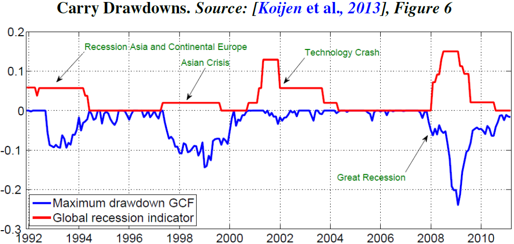
A similar drawdown dynamics is observed in every asset class: the downturn periods are closely associated with global recessions and liquidity crises.

6. SUMMARY

Carry is a component of total expected return, which can be measured in advance and does not require any knowledge of the 'true' model or data generating process. The key empirical facts about carry trade strategies can be summarized as follows:

1. High-minus-low carry portfolios generate positive risk-adjusted returns in various asset classes

2. Since carry reflects different aspects of returns for different asset classes, the returns on carry trade strategies are weakly correlated, thus providing diversification benefits for cross-class portfolio combinations

3. Nevertheless, the downside component of carry returns is similar for all asset classes --- carry trade losses coincide with global economic downturns and liquidity crunches

4. Carry is capable of predicting returns both in time-series and in cross-section (see section 3 in Koijen et al. (2013) [1] for further discussion)

References

- Carry,
, (2013)
- Options, futures, and other derivatives,
, (2006)
- Forward and spot exchange rates,
, Journal of Monetary Economics, Volume 14, p.319–338, (1984)
- Infrequent portfolio decisions: A solution to the forward discount puzzle,
, The American Economic Review, Volume 100, p.870–904, (2010)
- The cross section of foreign currency risk premia and consumption growth risk,
, The American economic review, Volume 97, p.89–117, (2007)
- Commodity trade and the carry trade: A tale of two countries,
- On the timing and pricing of dividends,
, The American economic review, Volume 102, p.1596–1618, (2012)
- The dog that did not bark: A defense of return predictability,
, Review of Financial Studies, Volume 21, Number 4, p.1533–1575, (2008)
- Stock return predictability: Is it there?,
, Review of Financial Studies, Volume 20, Number 3, p.651–707, (2007)
- Common risk factors in currency markets,
, Review of Financial Studies, p.hhr068, (2011)
- Carry trades and global foreign exchange volatility,
, The Journal of Finance, Volume 67, p.681–718, (2012)
- Countercyclical currency risk premia,
, Journal of Financial Economics, Volume 111, p.527–553, (2014)
- Value and Momentum Everywhere,
, The Journal of Finance, Volume 68, Number 3, p.929–985, (2013)
- Time series momentum,
, Journal of Financial Economics, Volume 104, Number 2, p.228–250, (2012)
- Log in to post comments