1. INTRODUCTION

Evaluating the return of an investment without proper accounting for risks taken does not make a lot of sense. Thus in asset management we take a relative performance perspective comparing the return on investment to return on investment with similar risk. Alpha is the average return in excess of such a benchmark (in other words speaking of alpha without properly defining the benchmark is meaningless). It is important that the benchmark should be tradable, furthermore, in practice it is usually a passive strategy (e.g. an index tracking ETF) which suggests little to no investment management and is affordable at reasonable price.

2. MEASURING ALPHA

Sticking to the Ang (2014) [1] notation we write the excess return as the difference between returns on asset and benchmark:

$r^{ex}_t = r_t - r^{bmk}_t\tag{1}$

Alpha is the average excess return across $T$ observations:

$\alpha=\dfrac{1}{T}\sum\limits_{t=1}^{T}{r^{ex}_t} = \dfrac{1}{T}\sum\limits_{t=1}^{T}{(r_t - r^{bmk}_t)}\tag{2}$

So far we did not look at risk. Consider an example of benchmarking against risk-free rate: alpha is then equivalent to the average risk premium $\alpha= \bar{r}_t - \bar{r}_{ft}$, and the Sharpe ratio is then $\frac{\alpha}{\sigma}$, where $\sigma$ is risk premium's standard deviation (which is equal to the standard deviation of asset return if the risk-free rate is constant). The information ratio generalizes Sharpe ratio for any benchmark:

$ IR=\dfrac{\bar{r}_t - \bar{r}^{bmk}_t}{\sigma(r_t - r^{bmk}_t)}=\dfrac{\alpha}{\bar{\sigma}}\tag{3}$

The denominator in (3) is called the tracking error, it measures the dispersion of asset returns around the benchmark. Just as the Sharpe ratio, equation (3) is interpreted as the excess return per unit of risk - in other words, how attractive investment is, accounting for the risk taken.

3.ADJUSTING FOR FACTOR RISK

Recall that asset return may be represented as a collection of factors that capture systematic risks. In case of the CAPM, the systematic component of excess return is

driven by single factor --- the market risk premium:

$E[R_i]-r_f = \beta_i(E[R_M] - r_f)\tag{4}$

Rearranging equation (4) we can write the expected return of asset $i$ as the following linear combination of the risk-free rate and market portfolio:

$E[R_i] =r_f+\beta_i(E[R_M] - r_f)=(1-\beta)r_f+\beta E[R_M]\tag{5}$

The RHS of (5) is the replicating portfolio, it implies that holding $(1-\beta)$ dollars in risk-free asset and $\beta$ dollars in market portfolio gives the same expected return as investing \$1 in asset i. In practice we estimate factor-adjusted alpha by running the following regression:

$ R_{it}-r_{ft} =\alpha_i +\beta_i(R_{Mt} - r_{ft})+\varepsilon_{it}\tag{6}$

Suppose we benchmark performance of an asset against the market risk premium. In this case, alphas measured as average excess return (equation (2)) and estimated from equation (6) are equal only if $\beta=1$. In other words, failing to adjust for factor risk is equivalent to assuming that the asset and benchmark share the same risk structure, which is: i.) not generally true; ii.) more importantly, misleading for evaluating investment's performance.
 

The same approach applies for a multiple factor benchmark, for example, the Fama and French (2014) [2] 5-factor model nests the CAPM and Fama-French 3-factor models as special cases:

$R_{it}-r_{ft} =\underbrace{\overbrace{\alpha_i +\beta_{M,i}(R_{Mt} - r_{ft})}^\textrm{CAPM}+\beta_{SMB,i}SMB_t+\beta_{HML,i}HML_t}_\textrm{FF 3-factor}+\beta_{RMW,i}RMW_t+\beta_{CMA,i}CMA_t+\varepsilon_{it}\tag{7} $

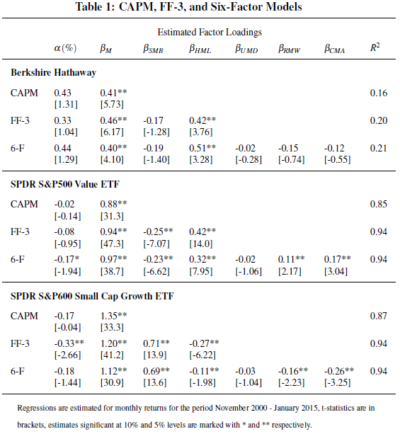
The RMW (robust-minus-weak) factor is constructed by buying (selling) stocks with robust (weak) profitability and reflect one of the quality's dimensions. CMA (conservative-minus-aggresive) takes long position in companies with low investments and shorts high investment firms. As an illustration consider a 6-factor model (FF-5 plus momentum) for Berkshire Hathaway and two ETFs, namely SPDR S&P500 Value (SPYV) and SPDR S&P600 Small Growth (SLYG). The estimates of regressions for monthly returns are displayed in Table 1, the sample is November 2000 - January 2015. The factors come from Kenneth French's page ( http://mba.tuck.dartmouth.edu/pages/faculty/ken.french/data_library.html).  

Moreover, we note that alpha is often expressed on annualized basis. An annualized alpha is thus simply obtained in case of the monthly regression by multiplying by 12, weekly alphas by 52 and so on.

4.GENERATING ALPHA

Active fund management is expected to deliver alpha in return for the higher costs typically charge. However, the average return for all investors cannot be better than the market return, adding the costs of management investors average returns have to be below market. Hence, it is often described as a losers game. Swedroe and Berkin (2015) [3] reflect on the possibility to generate alpha nowadays. The authors present four distinct reasons why they see higher hurdles of creating alpha in the future:

1. Alpha is measured with respect to factors carrying positive risk premia, hence, to create alpha fund managers need to exploit different strategies than just simply value, size, or momentum. Moreover, recently factor models incorporate more than just three factors, setting the hurdle even higher.

2. Untalented investors are increasingly shifting to pure passive strategies, due their poor performance. As a consequence, the set of remaining active managers becomes harder to beat due to the “adverse” selection.

3. Active managers follow an arms race by investing more in talent, data and technology. Developing new alpha generating strategies requires more and more resources.

4. The overall growth of assets implies that a fixed amount of money left at the table has to be divided in smaller pieces. (Even though it is hard to quantify)

5.SUMMARY

Alpha is just a mere reflection of a benchmark's factor composition. The benchmarks, however, should be tradable alternatives which are available to investors at low cost, so, for example, the CMA portfolio should not be included in benchmark, since there are currently no ETFs tracking this factor. Furthermore, benchmarks should be adjusted for risk, otherwise alphas will overstate performance relative to the risk taken, if the loading to the benchmark exceeds 1, and understate in the opposite case.
There are some additional issues that complicate performance evaluation. First, benchmarking against strategies with non-linear payoffs (think of derivatives) requires specific techniques. Second, factor loadings can vary over time, thus making proper adjustment for risk difficult --- so models allowing for dynamic loadings should be used (e.g. rolling regressions, dynamic conditional beta, or state space models, a short discussion on non-linear benchmarks and time-varying coefficients can be found in Ang (2014) [1] Ch.7).

References